手動でSuperlearner – Kentaro Kamada

文献

Naimi, Ashley I. & Laura B. Balzer, 2018, “Stacked Generalization: An Introduction to Super Learning,” European Journal of Epidemiology, 33(5): 459–64, (https://doi.org/10.1007/s10654-018-0390-z).

パッケージ読み込み

library(tidyverse)
library(rsample)
library(sl3)
library(future)
library(earth)

theme_set(theme_bw(base_family = 'Noto Sans JP'))

# 並列化
plan(multisession(workers = 5))

データ生成

\[\begin{align} Y = 5 + 4\sqrt{9x} \times I(x<2) + I(x\geq2) \times (|x-6|^{2}) + \epsilon \end{align}\]

\(I()\)：Indicator function（TRUEなら1、FALSEなら0となる）
\(\epsilon \sim \mathrm{Laplace}(0, 1)\)¹

set.seed(12345)

data <- tibble(
  x = runif(1000, 0, 8),
  epsilon = rmutil::rlaplace(1000, 0, 1)
) |> 
  mutate(
    y_truth = 5 + 4*sqrt(9 * x)*as.numeric(x<2) + as.numeric(x>=2)*(abs(x-6)^(2)),
    y = y_truth + epsilon
  )

データの確認（gamが優秀）

data |> 
  ggplot(aes(x, y)) +
  geom_point(alpha = 0.3)+
  geom_line(
    data = tibble(
      x = seq(0, 8, 0.1), 
      y = 5 + 4*sqrt(9 * x)*as.numeric(x<2) + as.numeric(x>=2)*(abs(x-6)^(2))
    ), 
    aes(x, y), 
    color = "black"
  )+
  geom_smooth(method = 'gam', formula = y ~ s(x, bs = 'cs'), se = FALSE)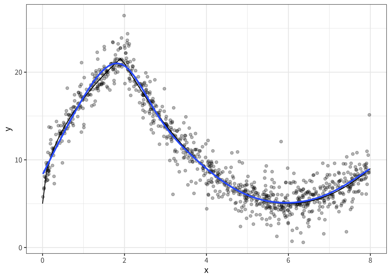

cross-fitの準備
データを5分割

df <- 
  vfold_cv(data, v = 5) |> 
  mutate(
    train = map(splits, analysis),
    test = map(splits, assessment)
  )

df

#  5-fold cross-validation 
# A tibble: 5 × 4
  splits            id    train              test              
  <list>            <chr> <list>             <list>            
1 <split [800/200]> Fold1 <tibble [800 × 4]> <tibble [200 × 4]>
2 <split [800/200]> Fold2 <tibble [800 × 4]> <tibble [200 × 4]>
3 <split [800/200]> Fold3 <tibble [800 × 4]> <tibble [200 × 4]>
4 <split [800/200]> Fold4 <tibble [800 × 4]> <tibble [200 × 4]>
5 <split [800/200]> Fold5 <tibble [800 × 4]> <tibble [200 × 4]>

手動でSuper learner

Cross-fitで各モデルの予測値を計算

res <- 
  df |> 
  mutate(
    model_earth = map(
      train, \(data) 
      earth(y ~ x, degree = 2, penalty = 3, nk = 21, pmethod = "backward", data = data)
    ),
    model_lm = map(
      train, \(data) 
      lm(y ~ poly(x, degree = 4), data = data)
    ),
    pred_earth = map2(model_earth, test, \(x, y) predict(x, newdata = y)[,1]),
    pred_lm = map2(model_lm, test, \(x, y) predict(x, newdata = y))
  )

各モデルの予測値を独立変数、アウトカムを目的変数とした回帰モデルを、Non-negative least squaresにより推定
パフォーマンスの良いモデルにより大きい重みがつくように、重みを推定

weight <-
  nnls::nnls(
    A = 
      res |> 
      select(pred_earth, pred_lm) |> 
      unnest(cols = c(pred_earth, pred_lm)) |> 
      as.matrix(), 
    b = data$y
  ) |> 
  pluck('x')

weight

[1] 0.2467513 0.5523356

# weightを、足して1になるように基準化
weight_normalized <- weight / sum(weight)
weight_normalized

[1] 0.3087915 0.6912085

予測値の計算

全データを用いて、各モデルの予測値を計算
先ほど推定した重みを用いて、各モデルの予測値を組み合わせた予測値を計算

# サンプル全体での予測値を計算
model1 <- earth(y ~ x, degree = 2, penalty = 3, nk = 21, pmethod = "backward", data = data)
model2 <- lm(y ~ poly(x, degree = 4), data = data)

result <- 
  data |> 
  mutate(
    pred1 = predict(model1)[,1],
    pred2 = predict(model2)
  ) |> 
  mutate(
    pred_sl = weight_normalized[1]*pred1 + weight_normalized[2]*pred2
  )

result

# A tibble: 1,000 × 7
       x epsilon y_truth      y pred1 pred2 pred_sl
   <dbl>   <dbl>   <dbl>  <dbl> <dbl> <dbl>   <dbl>
 1  5.77  -1.86     5.05  3.19   5.21  4.84    4.96
 2  7.01   1.16     6.01  7.18   6.36  6.57    6.51
 3  6.09  -4.30     5.01  0.712  5.16  5.00    5.05
 4  7.09  -0.353    6.19  5.83   6.56  6.75    6.69
 5  3.65   0.465   10.5  11.0    9.98 11.0    10.7 
 6  1.33  -0.677   18.8  18.2   20.0  19.5    19.7 
 7  2.60  -1.05    16.6  15.5   17.5  16.8    17.0 
 8  4.07   0.535    8.71  9.25   8.73  8.90    8.85
 9  5.82   7.05     5.03 12.1    5.20  4.85    4.96
10  7.92   2.30     8.68 11.0    8.52  8.20    8.30
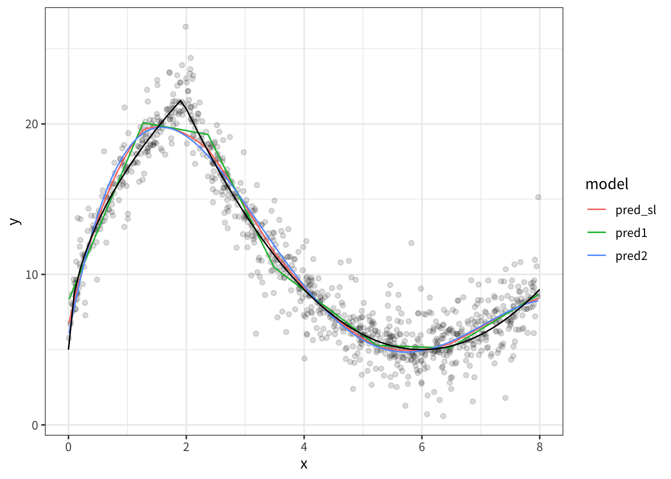
# ℹ 990 more rows

結果のプロット

result |> 
  pivot_longer(
    cols = c(pred1, pred2, pred_sl), 
    names_to = 'model', 
    values_to = 'prediction'
  ) |> 
  ggplot(aes(x, y)) +
  geom_point(alpha = 0.05)+
  geom_line(aes(x, prediction, color = model))+
  geom_line(
    data = tibble(
      x = seq(0, 8, 0.1), 
      y = 5 + 4*sqrt(9 * x)*as.numeric(x<2) + as.numeric(x>=2)*(abs(x-6)^(2))
    ), 
    aes(x, y), 
    color = "black"
  )

`sl3`でSuper learner

task <- sl3_Task$new(
  data = data, outcome = "y", covariates = "x", outcome_type = 'continuous', folds = 5
)

sl_lib <- 
  Lrnr_sl$new(
    learners = Stack$new(
      Lrnr_earth$new(degree = 4), 
      Lrnr_gam$new(),
      Lrnr_mean$new(),
      Lrnr_xgboost$new(nrounds = 100, max_depth = 3, eta = 0.3),
      Lrnr_bartMachine$new(serialize = TRUE)
    ),
    metalearner = Lrnr_nnls$new(convex = TRUE)
  )

fit <- sl_lib$train(task)

serializing in order to be saved for future R sessions...done
serializing in order to be saved for future R sessions...done
serializing in order to be saved for future R sessions...done
serializing in order to be saved for future R sessions...done
serializing in order to be saved for future R sessions...done
serializing in order to be saved for future R sessions...done

fit

[1] "Cross-validated risk:"
Key: <learner>
                           learner coefficients       MSE        se   fold_sd
                            <fctr>        <num>     <num>     <num>     <num>
1: Lrnr_earth_4_3_backward_0_1_0_0    0.0000000  2.439980 0.1491178 0.5590197
2:                 Lrnr_gam_GCV.Cp    0.6423803  2.156928 0.1368631 0.5163999
3:                       Lrnr_mean    0.0000000 30.590277 1.0519860 2.2451721
4:        Lrnr_xgboost_100_1_3_0.3    0.0000000  2.437071 0.1515221 0.5109703
5:           Lrnr_bartMachine_TRUE    0.3576197  2.215505 0.1425014 0.4516937
   fold_min_MSE fold_max_MSE
          <num>        <num>
1:     1.969880     3.393874
2:     1.767867     3.055205
3:    27.834174    33.991665
4:     2.098941     3.308421
5:     1.895672     3.001563

result |> 
  mutate(
    pred_sl3 = fit$predict(task = task)
  ) |> 
  pivot_longer(
    cols = c(pred1, pred2, pred_sl, pred_sl3), 
    names_to = 'model', 
    values_to = 'prediction'
  ) |> 
  ggplot(aes(x, y)) +
  geom_point(alpha = 0.05)+
  geom_line(
    data = tibble(
      x = seq(0, 8, 0.1), 
      y = 5 + 4*sqrt(9 * x)*as.numeric(x<2) + as.numeric(x>=2)*(abs(x-6)^(2))
    ), 
    aes(x, y), 
    color = "black"
  )+
  geom_line(aes(x, prediction, color = model))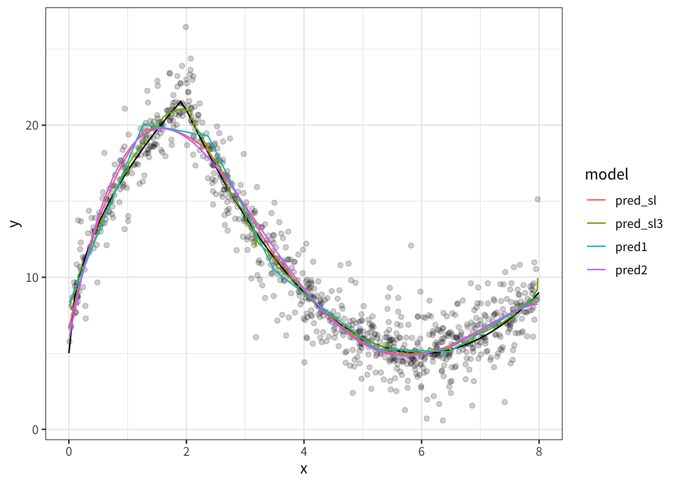

Footnotes

ラプラス分布。二重指数分布（double exponential distribution）とも呼ばれる。論文中ではdoubly-exponential distributionと表記されている。↩︎

文献