マルチレベルモデルは点推定値に影響を及ぼすか？

library(tidyverse)
library(lmerTest)
library(broom)
library(broom.mixed)

マルチレベルモデルにおけるよくある誤解

「マルチレベルモデルでやんなきゃ係数にバイアスが…」←ホント？

データ生成

マルチレベルのデータを考えるサンプルサイズ1000、グループ数50のデータ

\[\begin{align} y_{ig} \sim 0.5x_{ig} + \mathrm{Normal}(\theta_g, 1) \\ \theta_g \sim \mathrm{Normal}(0, 3) \\ x_i \sim \mathrm{Normal}(0, 1) \end{align}\]

dgp <- function(samplesize = 1000) {
  tibble(
    id = 1:samplesize,
    group = rep(1:50, 20),
    x = rnorm(samplesize, mean = 0, sd = 1),
  ) |> 
    group_by(group) |> 
    mutate(group_mean = rnorm(1, mean = 0, sd = 3)) |> 
    ungroup() |> 
    mutate(y = 0.5*x + rnorm(samplesize, mean = group_mean, sd = 1))
}

data <- dgp()

lm(y ~ x, data = data) |> 
  summary()


Call:
lm(formula = y ~ x, data = data)

Residuals:
    Min      1Q  Median      3Q     Max 
-9.9673 -2.3079  0.2522  2.4065  7.8351 

Coefficients:
            Estimate Std. Error t value Pr(>|t|)  
(Intercept)  0.01677    0.10746   0.156   0.8761  
x            0.21591    0.10766   2.005   0.0452 *
---
Signif. codes:  0 '***' 0.001 '**' 0.01 '*' 0.05 '.' 0.1 ' ' 1

Residual standard error: 3.398 on 998 degrees of freedom
Multiple R-squared:  0.004014,  Adjusted R-squared:  0.003016 
F-statistic: 4.022 on 1 and 998 DF,  p-value: 0.04518

lmer(y ~ x + (1|group), data = data) |> 
  summary()

Linear mixed model fit by REML. t-tests use Satterthwaite's method [
lmerModLmerTest]
Formula: y ~ x + (1 | group)
   Data: data

REML criterion at convergence: 3144.8

Scaled residuals: 
    Min      1Q  Median      3Q     Max 
-3.4810 -0.6754  0.0040  0.7066  3.4708 

Random effects:
 Groups   Name        Variance Std.Dev.
 group    (Intercept) 10.767   3.281   
 Residual              1.038   1.019   
Number of obs: 1000, groups:  group, 50

Fixed effects:
             Estimate Std. Error        df t value Pr(>|t|)    
(Intercept)   0.01684    0.46517  48.99703   0.036    0.971    
x             0.46739    0.03312 949.48170  14.111   <2e-16 ***
---
Signif. codes:  0 '***' 0.001 '**' 0.01 '*' 0.05 '.' 0.1 ' ' 1

Correlation of Fixed Effects:
  (Intr)
x 0.000

シミュレーション

データを1000個作成

data_list <- 
  map(1:1000, \(x) dgp(1000)) |> 
  enframe()

OLSと変量効果モデルで推定

result <- 
  data_list |> 
  mutate(
    lm = map(value, \(data) lm(y ~ x, data = data)),
    lmer = map(value, \(data) lmer(y ~ x + (1|group), data = data))
  )

xの係数のみ取り出す

res2 <- 
  result |> 
  mutate(
    lm_res = map(lm, \(model) {
      tidy(model) |> 
        select(term, estimate)
    }),
    lmer_res = map(lmer, \(model) {
      tidy(model) |> 
        select(term, estimate)
    })
  ) |> 
  select(name, lm_res, lmer_res) |> 
  pivot_longer(!name, names_to = 'model', values_to = 'value') |> 
  unnest(value) |> 
  filter(term == 'x')

結果を図示

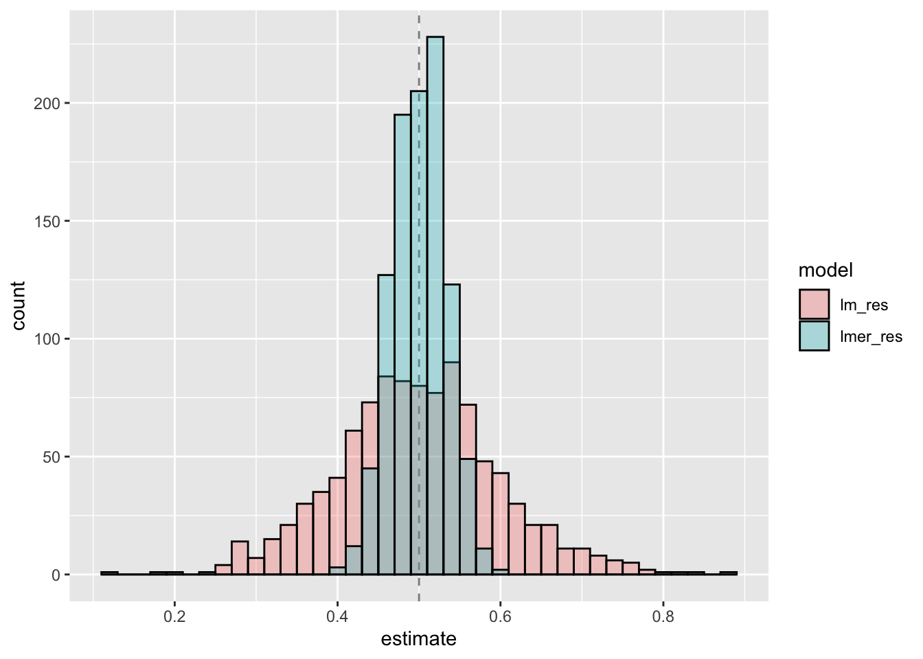
どちらの点推定値も真の値の0.5を中心に分布＝バイアスはない
OLSによる点推定値はバリアンスが大きい
変量効果（マルチレベル）モデルによる点推定値はバリアンスが小さい

res2 |> 
  ggplot(aes(estimate, fill = model))+
  geom_vline(xintercept = 0.5, linetype = 'dashed', alpha = 0.5)+
  geom_histogram(alpha = 0.3, color = 'black', binwidth = 0.02, position = 'identity')+
  scale_x_continuous(breaks = seq(0, 1, 0.2))